Math Modeling: Day 39

• I highlight, in bold, the important piece which the university isn't highlighting in the FAQ for students....

1. Today, Wednesday: How we might simulate a time series, like temperatures, based off the variogram.

2. Friday: Review for the final

We model that correlation using the "empirical variogram" (a temporal decomposition of the sample variance), constructing something we call the "theoretical variogram".

We find roughly the same thing for our data, especially after having removed the trend (which you should have calculated for homework) for the two time series:

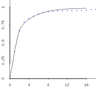
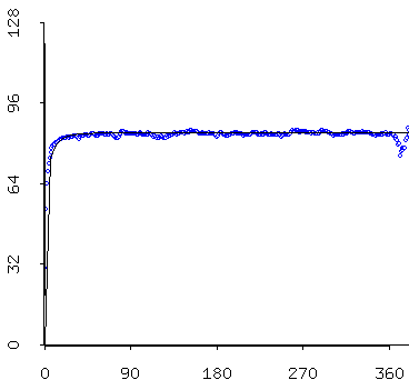
At left: zooming in on the nose of the graph at right.	The "empirical variogram" and the "theoretical variogram for the residuals of the minimum temperature model (after we've removed your models).

I mentioned last time that we want to render our data "stationary" before we simulate. In order to do that, we need to take care of some issues in our mins and maxes: their fluxuating means and standard deviations.

When I talk about their means and standard deviations, these refer to the distribution of values we see for each day of the year over 127 years or so of BG weather. Consider August 15th, for example, and the minima. If we plot them for the 127 years, we see a distribution like this:

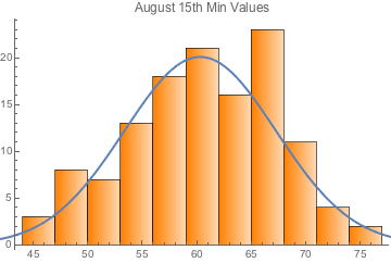
Empirical PDF -- Probability Density Function -- for August 15th Minima with a suggested normal-distribution overlay. Maybe the data isn't normal, but that's just to give you the idea.

For each day we have a mean minimum, and a standard deviation of the minima. So those are the values that were plotted above, for the whole year.

We might want to create a theoretical distribution from the empirical data -- otherwise we'd never be able to exceed the extremes of the data (to "create new records").

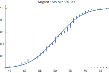
Empirical CDF -- Cumulative Distribution Function -- for August 15th Minima with a normal cdf overlay (I just used the mean and the standard deviation of the empirical data to estimate the normal). Maybe the data isn't normal, but this is just to give you the idea. By the way, for the randomin

If we look at the distribution of means and standard deviations of these temperatures across the year, over 127 years:

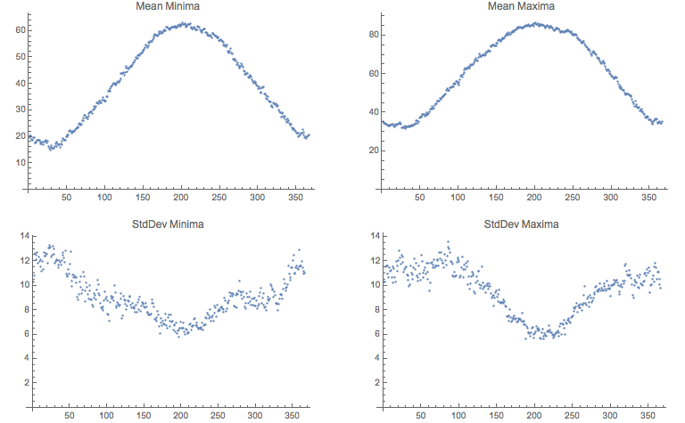
In the summer months, the deviation is lower; in the winter the deviation is higher.

But only roughly like a sinusoid: so we regress with a few more periods (here's the Mathematica code, and a pdf of the output) to capture some of the dramatic wiggling in the standard deviations (in this case I used sines and cosines with terms $\cos(2\pi x), \cos(4\pi x), \ldots, \cos(12\pi x)$, and corresponding sine terms).

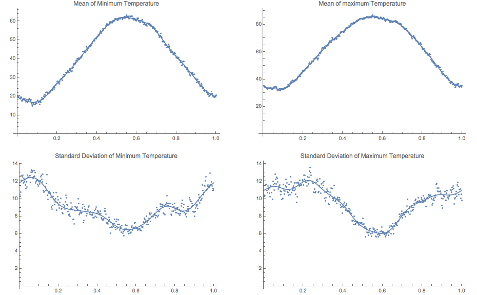
These terms correspond to the following:

Now we re-standardize the data, using these functions of time (e.g. MinMean(t), MinSD(t)), where these are annual function, with period one year: for each minimum value $min(t)$ from the BG data set, standardize it via \[ Zmin(t)=\frac{min(t)-MinMean(t)}{MinSD(t)} \]

I call it $Zmin$ because it's roughly mean 0, standard deviation 1 -- like a standard $Z$. But this $Zmin$ is still autocorrelated.

For example, check out 3/8/47 in the data as it arrived from NOAA.

What do you notice?

1947     3        8  
1957     11       13 
1982     6        1  
1985     2        23 
1994     1        16 
1994     1        19 
1994     1        20 
1996     6        21 

So we try to find anything like this -- obvious data errors -- which will cause trouble for our analysis.

It has been quite the labor of love -- no, not love, but rather pain -- to trick gstat into doing what I wanted. But, in the end, it seems to have worked. gstat is designed for spatial situations, so it assumes two spatial dimensions -- so I created a constant coordinate to add to time, to trick it: $(1,1), (2,1), (3,1), \ldots, (45782,1)$.

Now I use R and RStudio to compute the variogram, and (attempt) to fit a model -- but it didn't do as well as my other software, so I did that myself and handed it to gstat. Except that we evidently disagree on some definitions, so... at any rate, I'm getting pretty close, with some educated guessin:

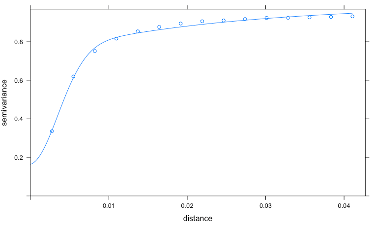
So if we're going to simulate a temperature (let's say a min), you

1. Standardize the data, creating $Zmin$ as described above: \[ Zmin(t)=\frac{min(t)-MinMean(t)}{MinSD(t)} \]
2. Compute the empirical variogram for $Zmin$.
3. Model the empirical variogram with a theoretical variogram:
   

   Again, just to emphasize: this is a non-linear regression problem, with a family of functions that have properties essential for the job of modeling what is essentially a variance.

4. Pass that model to gstat.
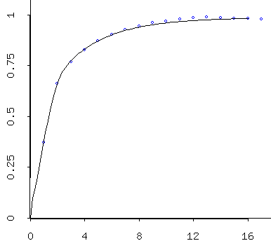
5. Have it generate simulations on the same dates that we have for our data, which have the same temporal autocorrelation structure as $Zmin$ (it's hard to tell the difference between the one below (simulation) and the one above (Zmin), isn't it?):
   

6. Un-Standardize the data, creating $Smin$ by undoing what we did to create $Zmin$, but on the simulated data $simZmin$: \[ Smin(t)=simZmin(t) MinSD(t) + MinMean(t) \]

7. Associate the years with this data set, as though it were "Bowling Green temperatures"

   Here's the result of regressing the simulated minima and the actual minima against $\sin(2 \pi t)$ and $\cos(2 \pi t)$:

   (and, by the way, my results will be slightly different from yours, unless you too removed some erroneous data -- maybe you found some more erroneous data to remove...!:)

   Linear Regression: Estimate SE Prob Constant 40.0818 (4.257565E-2) 0.00000 Variable 0 -20.4231 (6.012267E-2) 0.00000 Variable 1 -8.29364 (6.029912E-2) 0.00000 R Squared: 0.746108 Sigma hat: 9.10964 Number of cases: 45782 Degrees of freedom: 45779	simulated minima $Smin$: Mean: 40.017 SD: 18.079
   Linear Regression: Estimate SE Prob Constant 40.0546 (4.318030E-2) 0.00000 Variable 0 -20.9435 (6.097651E-2) 0.00000 Variable 1 -7.24789 (6.115547E-2) 0.00000 R Squared: 0.742800 Sigma hat: 9.23901 Number of cases: 45782 Degrees of freedom: 45779	actual minima Mean: 39.993 SD: 18.217
   Linear Regression: Estimate SE Prob Constant 60.6425 (4.549809E-2) 0.00000 Variable 0 -24.7985 (6.424956E-2) 0.00000 Variable 1 -9.12010 (6.443812E-2) 0.00000 R Squared: 0.787120 Sigma hat: 9.73493 Number of cases: 45782 Degrees of freedom: 45779	simulated maxima $Smax$: Mean: 60.567 SD: 21.099
   Linear Regression: Estimate SE Prob Constant 60.6009 (4.605287E-2) 0.00000 Variable 0 -25.3769 (6.503299E-2) 0.00000 Variable 1 -7.87640 (6.522385E-2) 0.00000 R Squared: 0.784930 Sigma hat: 9.85363 Number of cases: 45782 Degrees of freedom: 45779	actual maxima Mean: 60.530 SD: 21.247

8. Compute the extreme year data (i.e. the "Fletcher data").

   (to come!)

9. Now do it 1000 times....

10. Compare the Fletcher data to the range of possible distributions obtained by simulation, to see how likely (or unlikely) it would be, assuming no climate change.

    (Because our model has no climate change in it: the same means and standard deviations repeat year after year....)