Exploratory Spatial Data Analysis and Scientific Visualization

1. 1-d, 2-d, 3-d, and beyond
   1. Histograms, boxplots, scatterplots, etc.
   2. Two and three dimensional plots
   3. Functions from points: interpolation and smoothing
   4. Time: adding a fourth dimension
2. Seeing (and quantifying) spatial autocorrelation
   1. The spatial autocorrelation game
   2. BW (Black/White) statistics
   3. variograms
3. Summing up

The data for many of these plots is two dimensional nitrate data from water wells sampled in the area around Phoenix, Arizona. Nitrate has been linked to health problems in infants, for example ("Blue babies"). One of the problems we faced in analyzing this data was to plot it in a meaningful way; another was to create a map of nitrate concentration for the whole study area (interpolation, extrapolation), based on the point data.

1. 1-d, 2-d, 3-d, and beyond

   1. Histograms and boxplots are essentially one-dimensional representations of data. They allow you to gather information about the distribution of a single variable. Linked with other plots, however, they can provide much more information.

   2. Two and three dimensional plots

      1. Often the first thing we do with spatial point data is create a scatterplot of the study region.

      2. Color helps one gauge the variation in a variable over the map, just as it does for choropleth maps of polygon data (wherein color is used to categorize the areas according to an attribute of the area).

         Dr. Cynthia Brewer of Penn State has prepared a nice web page on Color Use Guidelines for Mapping and Visualization. Please take a look at it, and click on some of the color schemes (the graphics) to see the example choropleth maps associated with them.

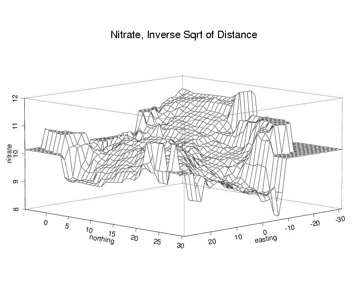
      3. Elevation is another means for helping gauge variation, but it can be confusing unless we add other clues (for example rotation, or stereo). Note the use of labels in this plot: the labels actually serve as an additional dimension of information!

      4. Stereo helps us to see in higher dimensions, if you know how to use it!

      5. Symbol size variation and type, like color, permit us to get a gross impression of additional variation. This may be achieved via brushing and spinning as an aid to seeing in high dimensions and/or identifying outliers.

   3. Functions from points: interpolation and smoothing (splines, smoothing with kernels) - creating continuous functions from scattered data (naively).

      1. one-d - e.g. splines, lowess, kernel smoothing, inverse distance weighting....

         The general idea of all these techniques is that you estimate at a point away from the data locations by using a weighted sum of neighboring values. The issue then is generally of two forms: how do you define a neighbor, and what weights do you attribute to them?

         We're primarily interested in (at least) two dimensions, but it's easier to explain things in one dimension, so we'll start there. These naive schemes are essentially ad-hoc, and their use is somewhat questionable. Each implies spatial autocorrelation, which may or may not have been tested. It's easy to hit the button that says "interpolate"! If you believe, however, that a smooth function underlies the point data given the phenomenon you are examining, then you are safe in assuming some degree (but how much?) of spatial autocorrelation. That's why we talk about quantifying spatial autocorrelation.

         Here are random data "smoothed" when they never should have been:

         • kernel-smoothed
         • spline-fit (an interpolator - "interpolators" are functions constrained to pass through the data points - but do you really want to do that?)
         Kernel and lowess smoothing and spline-fitting procedures (e.g. those you find in SAS or S-PLUS) usually offer the user choices, such as the number of neighbors to include in processing, the type of "kernel smoother", the power on the inverse distance weighting, etc. These choices are part of the ad hoc nature of these routines.

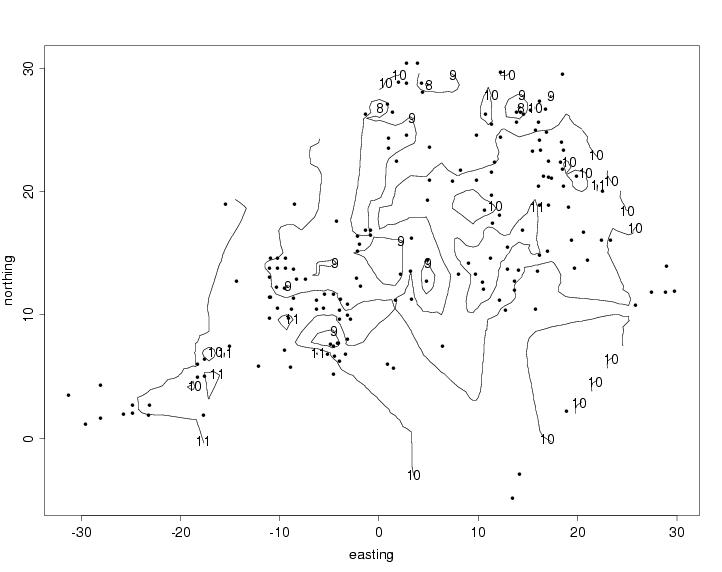
      2. two-d - As a precurser to contour plots and image plots

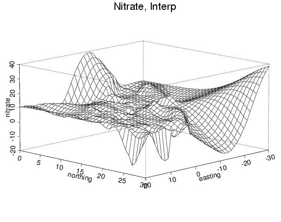
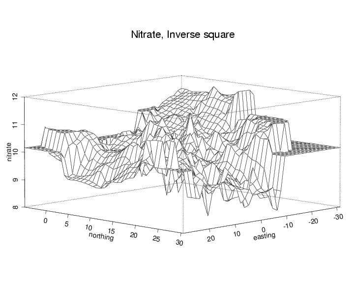
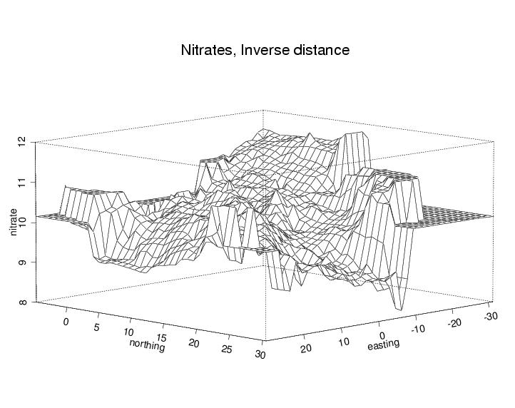
         It is important to realize that contour plots from data scattered in space are based on an interpolation step (that is, first a grid of values has to be calculated from the scattered values). One traditional method of doing this is inverse-distance weighting: that is, the weight associated with a neighbor falls off as a function of distance.

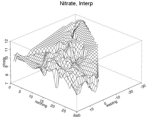
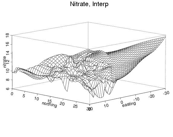
         Here are some perspective plots created using S-PLUS. The first set is obtained using S-PLUS's native "interp" program (i.e., the user asked no questions, but just had S-PLUS do its thing):

         • no extrapolation (this means that away from the data points the method will not make estimates)
         • extrapolation - wild! The method estimates, even far from the data.
         • again, extrapolation (a little saner?)
         The other three are obtained by using various degrees of inverse distance weighting:
         • 1/d^2
         • 1/d
         • 1/sqrt(d)
         Other methods exist for indicating the third dimension, yet present the data projected onto the two-dimensions of the page.
         • contour plots, and
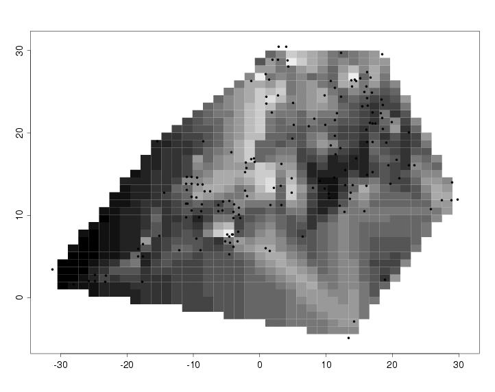
         • image plots,
         both based on the native interp interpolator without extrapolation of S-PLUS.

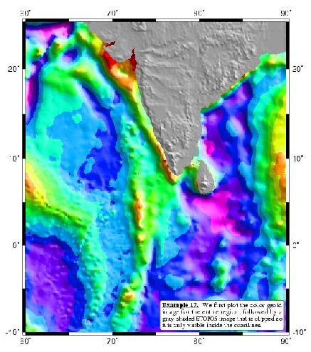
         James A. Wood interpolated his data to create this map of brush fire history. Not to take anything away from Mr. Wood, but we're not told what method he used to do his interpolation....

         Raster maps (whether created by using interpolated data, or by remote sensing data as we see here) can look very beautiful, indeed! Of course the proper choice of color scheme again plays a big role.

   4. Time is a wonderful way to add a fourth dimension.
      1. Putting a series of point plots into an animation is becoming increasingly easy, as we see in this map of changing U.S. population.

      2. In this case it stands for a parameter which is varying in a model for interpolation weights (we're getting to that in a second!);

      3. In these rabies time series animations we can watch as an epidemic spreads over the face of Connecticut.

         One difference between these rabies animations and the animation of population above is the method: Javascript versus animated gif images. Both methods are easily within the grasp of interested students.

2. Seeing (and quantifying) spatial autocorrelation

   We all are already experts at using the "visual metric" (or visual measuring stick): the eye is the champion pattern identifier. However, some folks are better at it than others, and the eye may find patterns where none exist. For this reason, Geoff Jacquez warns often of the "Gee Whiz" effect, which he defines as follows:
   'The "Gee Whiz" effect proceeds as follows. First, spatial data are manipulated using a GIS to generate thematic maps that may be quite striking in appearance. After all, the maps we choose to display to our colleagues are those that do the best job of illuminating possible spatial relationships! The map stimulates our thinking, and we formulate a plausible cause for the disease pattern. The "Gee Whiz" effect occurs when we undertake an intervention based on this explanation.'

   1. If you haven't already, play the Spatial Autocorrelation Game

      What does spatial autocorrelation look like? How did you know when you'd gotten large positive or large negative values? (Here are some examples of extreme spatial autocorrelation.) In this game, spatial autocorrelation was measured by the global measures of Moran's I and Geary's C (the precise definitions can be found from the documentation for the SA Game). Thus, a single number is used to capture global spatial autocorrelation for a data set (or an image, in this case).

      There are several common, different ways of measuring spatial contiguity (who are my neighbors?): Rook, Bishop, and Queen. The Spatial Autocorrelation game uses the Rook's definition. Each definition gives rise to different values of statistics, and different conclusions (perhaps) about the degree of spatial autocorrelation.

   2. BW (Black/White) statistics - binary data

      In lab we have looked at choropleth maps of cancers. The colors were related to the cancer rate. BW statistics work in simpler situations: where we have a binary response (e.g. disease in an area or no; or above the median or below it). Example: Snow's Data.

      These statistics are useful on areas, and on sites converted to areas via Theissen polygons, which permit us to create a definition of contiguity between sites. Starting with point data, regions are defined which are effectively "basins of attraction". If you look closely at the plot of the Theissen polygons, you'll see that the region surrounding a given point is filled with the points in the study area closer to that point than to any other in the data set.

      In your reading is the derivation of the BW z-statistic (Cliff, A. D. and P. Haggett. 1988. Atlas of Disease Distributions: Analytic Approaches to Epidemiological Data. Blackwell, Ltd., Oxford, UK. Pages 33-35.). Those authors also give us a way of interpreting the BW statistic, based on the sign of that statistic (basically BW-E(BW)):

      • Negative:
        1. disease spread from few sources
        2. large areas favoring similar disease levels
        3. gradient or trend in disease intensity across maps
      • Positive:
        1. heterogeneous study area
        2. small areas favoring similar disease levels
      For Snow's data, the BW statistic was -3.02.

      Cliff and Haggett refer to the "connection matrix", which expresses the contiguity of neighboring regions (whether they are adjacent or not). In the case of a large number of regions, this is non-trivial to calculate: that's where GIS can help, as some GIS utilities are able to provide this information (e.g. Luc Anselin's SpaceStat extension or Dan Griffith's extension to ArcView).

   3. variograms

      We'll be getting into "variography" more heavily in the geostatistics module, when we talk about geostatistics in some detail, but a brief and qualitative introduction to the basic concept may be appropriate.

      Certainly one can imagine that a single number may not capture the range of spatial autocorrelation in a data set. For example, positive spatial autocorrelation may fall off as some function of distance, and the appearance of the data will presumably change as this function changes.

      Thus a single number (e.g. Moran's I) may not give us a sufficiently broad picture of the spatial autocorrelation; it may be that a function would give us more detailed information about the pattern. An example of such a function is the variogram.

      The variogram is another measure of spatial autocorrelation (another of the "signatures" that Geoff has talked about in a previous module), composed essentially of estimates of variance in different classes. We divide all pairs of data points into disjoint classes (that is, each pair belongs to only one class), and then we average over each class, generally plotting the result. In this example, the bins were created using inter-point distance.

      1. The sample variogram is a spatial decomposition of the sample variance (heavy math section! Only for the brave). That is, we compare pairs of points, squaring their differences, but rather than simply taking their mean, we put the pairs into bins according to distance and angle, and represent each bin by its mean. If there is no distance/direction effect, then there will be only random differences in the bin values; on the other hand, if there is a systematic difference, we will want to characterize it (the role of the theoretical variogram).

         Here are some other examples of variograms:

         • Abe Lincoln and his variogram. In this case the data set is composed of the pixels of the image (or rather, the image is the representation of a gridded data set); and
         • an example of the variogram cloud for a spatial point data set. This is more typical of the kinds of data you will have. This latter image shows how one group at Iowa State has created an interface between ArcView (UNIX version) and XGobi to permit spatial analysis.

      2. A variogram that is "flat" (i.e. the same across bins) tells you that you needn't worry about spatial autocorrelation (at the scale examined). For example, in a previous module I used inverse distance weighting to interpolate the FIPS codes of counties of Illinois. If I had looked at the variogram of FIPS, I'd have known that that was a bad idea (remember, the FIPS code possesses no spatial information): not only is the variogram essentially flat, but it appears to be higher at the small distances, which says that nearer neighbors are to be trusted less than far ones!

3. Summing up

   Visualization is an important and perhaps under-utilized component of many analyses. It may lead to hypothesis generation, confirm or defy expectations, and aid in the presentation of results you've obtained. The use of color, symbol, symbol size, stereo, and time may aid in presenting higher dimensional results, and the linking of brushing of plots may also enhance the information content of plots.

   Most packages allow for the choice of color, symbol, and symbol size when making plots; other options are a harder to find in most software, but we have seen examples of their use. Many useful public domain packages such as Xlispstat and XGobi provide brushing, as do commercial packages such as S-PLUS. Stereo is hard to come by, as is the creation of movies of your images. Look to the future for those options, although options such as the Java language within web pages make animation easier (as we saw in the rabies animations above).

   Spatial autocorrelation is important, both as a factor in the study of a disease (i.e. is it likely to spread?) and as a characteristic to be exploited when mapping disease. Traditional techniques include single statistics such as Moran's I, or Geary's C, and black and white statistics; we saw that a non-traditional spatial statistic called the variogram can be used to actually model spatial autocorrelation.

   Now that you're done:
   • Try the lab!
   • Additional Readings
   • Please: evaluate this module. We appreciate your comments!
   • Back to the
     

Page by Andy Long. Comments appreciated.