Math Modeling: Day 33

1. Question: I have a couple questions about what the upcoming exam will look like on Friday. I saw online that there will be a timed and a take home portion, but I wasn't really sure what a timed portion would look like. Will you just send us the exam and expect us to have it emailed to you or put into our Google Drive folder within the hour of the class time, or something else?
   Answer: That's it -- an hour to do a part, and then some time to deal with the "take home" part -- perhaps til Sunday eve. I'll probably just put a link to the exam on the website. You can either work on a paper copy, or work on scratch paper -- then you'll email me your exam (or put it on your folder, and let me know it's there).

These are the sinusoidal models of Fletcher's BG Climate Normals, by month (max, mean, min temperatures), plus a model for all the 1893-1992 record temperatures taken from the Fletcher data.

• Sean's versions
• And now, for more than you probably want to see... :)
  1. FletcherMinMaxMeanSinusoids.nb
  2. FletcherMinMaxMeanSinusoids.pdf

1. Predator/Prey:
   1. Lab 1: logistic and intro to InsightMaker

   2. Lab 2:
      1. Basic predator/prey model (Lotka-Volterra)

   3. Lab 3:
      1. Tyson et al. Lynx and Hare
      2. Samuel did a nice job on PP3

2. SIR models:
   1. Lab 1:
      1. Basic SIR model
      2. Jacob A. did a nice job on SIR 1

   2. Lab 2:
      1. SIR model with Death (SIRD: flatten the curve)
      2. Proctor did a nice job on SIR 2

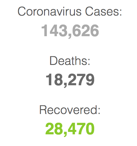
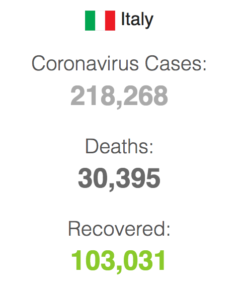
   3. Lab 3: SIR model of Covid-19 in Italy

      Proctor did a nice job on SIR 3

      Our model predictions for Italy, May 9th:

      1. Total cases: 214K (actual: ... to come!)
      2. Deaths: 37.4K (actual: ... to come!); as of April 9th, we had Click that image for an update. [ael: I've updated as of the 10th of May:]
         

Here are some regression results from Mathematica:

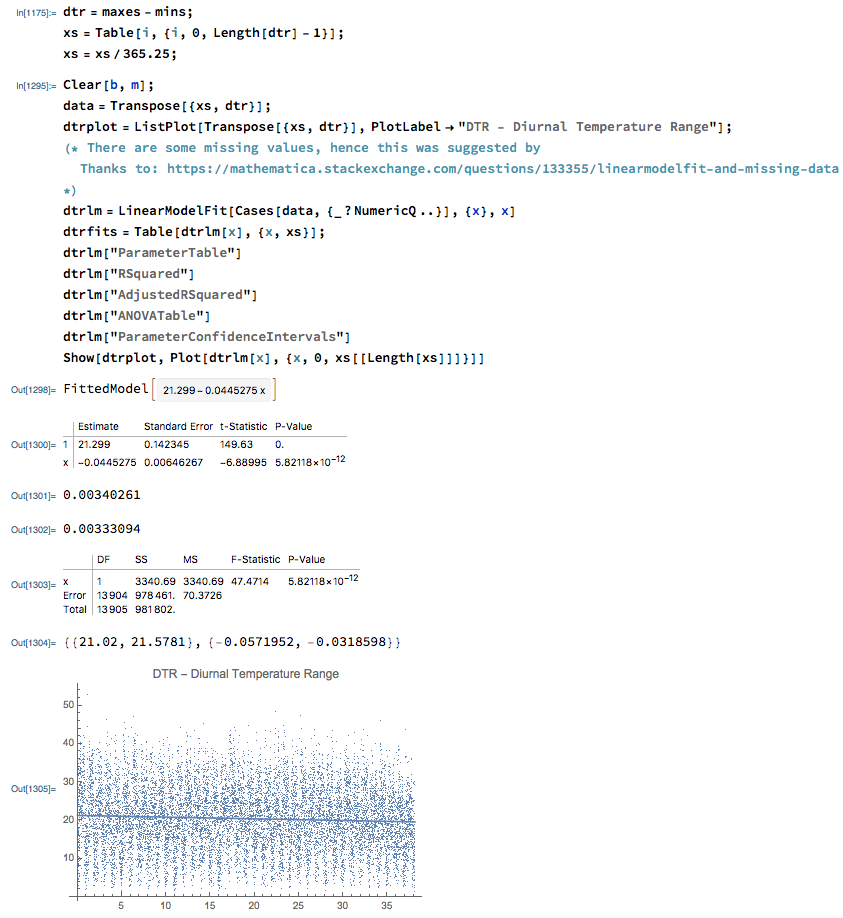
Let's take a moment and look over these results. Some observations:

1. As I mentioned in an email, Mathematica didn't know how to handle the missing values, so barfed on

   		dtrlm = LinearModelFit[data, {x}, x]
   		

   Silas and I had to remove some missing values, which led to the ugly regression command

   		dtrlm = LinearModelFit[Cases[data, {_?NumericQ ..}], {x}, x]
   		

   Mathematica strips off any non-numeric cases. There is nothing I can say about that command -- it's completely non-intuitive -- but I can say that I found it by googling something like "Mathematica handle missing cases regression" (or the like), and then looking for something from stackexchange

   (* There are some missing values, hence this was suggested by
   Thanks to George2079: 
   https://mathematica.stackexchange.com/questions/133355/linearmodelfit-and-missing-data
   *)
   

   (I always try to embed "credit where credit is due" in code.)

2. Now, in terms of diagnostics:
   1. Linear regression will always produce a fit (in this case $DTR(x)=21.299-.0445275x$) -- but is it any good?

   2. The adjusted $R^2$ is .00333094 -- which doesn't sound very good! But look at that data -- does it look like a straight line is going to capture much of that wildly wiggly variation?:)

      By the way, better to use "adjusted" $R^2$ because it penalizes a model for using more parameters -- we can always get a better fit by adding an additional parameter. So you're basically saying how much additional bang do I get for that extra parameter?

      So what we focus on here is a different question: is the slope significantly different from zero?

   3. The slope parameter (coefficient of $x$) has a p-value of $5.82118x10^{-12}$. Probably less than any $\alpha$...:) It says there is really a negative slope to this data.

   4. The confidence interval says the same thing: $m \in \{-0.0571952,-0.0318598\}$, with 95% confidence. We are certain that it's negative.

   5. So the conclusion is that this data -- which we think of as a surrogate for Fletcher's data -- shows that the Diurnal Temperature Range (DTR) has, in fact, decreased over the 38-year period, from 1982 to 2020.

Fletcher stuff may appear as well. You should try to be up to speed on everything we've been doing, especially since Spring Break. I know that it's been rougher for some of you than for others.

There may be an InsightMaker component. That would seem reasonable, given all we've done.

1. Newton's method:
   

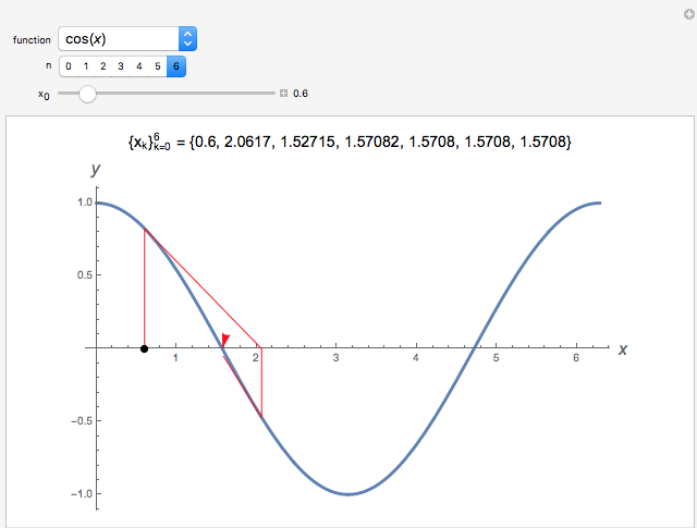
   Newton's method is a powerful numerical technique for solving the important (but trivial looking) equation \[ f(r)=0 \] for the "root" $x=r$. There may be no solution; there may be an infinite number of solutions (as in the example shown in the figure above).

   Newton's method is iterative: that is, we start, do it once, and then restart, doing it again and again (until satisfied). In the end we have only an approximate root, but we hope that it suffices for our purposes: so do this, starting from your good guess $x_0$, until satisfied (let's say $N$ times):

   \[ x_{n+1}=x_{n}-{\frac {f(x_{n})}{f'(x_{n})}} \] Then take $r \approx x_N$.

   This is not an easy problem, in general, but with a good starting guess, and a little luck (plus the ability to compute derivatives) we may be able to find a useful root.

2. Non-linear regression -- examples (e.g. Cadavars, Corn Growth)

   Non-linear regression is frequently done by simply iterating linear systems. It's a really cool example of a generalization similar to Newton's method. The trick is starting with a good guess.

   • We saw that, when we allowed Mathematica to start looking for a function of the type specified for the cadavar problem, that it came up with a really ugly "solution":
     

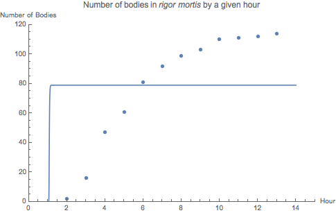
     But, when we gave it a little guidance (using some good approximations, some obtained by "almost linearizing" the system), the solution obtained and shown here --

     
     is a very pretty function, which we can then use in forensic science to predict how long a person has been dead, say.

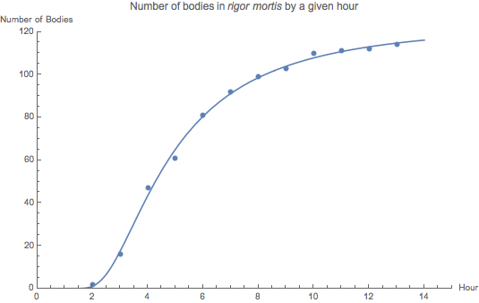
     Our job as a math modeler is frequently to fit data. There is often a "part 2", however: for example, now predict a value outside of the data set (extrapolation), or between data points (interpolation).

   • Similarly, we saw in the case of some corn-growth data that exponential models made no sense, and so we tried a logistic function to fit this:
     

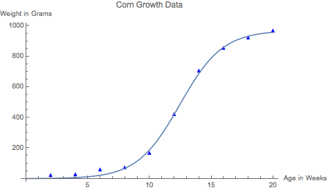
     That made more sense, as the corn should asymptote, which the logistic function does.

3. Our next topics were differential equations, and we talked about some simple examples:

   • \[ \frac{dy}{dt} = \alpha y(t) \] The general solution method is to stare at one until the solution comes to you -- although numerics are also an option (such as we saw for the solution of the root problem with Newton's method).

     This one says "do you know a function which is its own derivative up to a constant?" And there are two good answers: an exponential function, and $y(t)=0$. But the exponential turns out to be a lot more useful for modeling populations....

     Usually we also provide an initial condition - $y(0)=y_0$ -- so that the solution is uniquely determined for all time: \[ y(t)=y_0 e^{\alpha t}. \]

     If $\alpha > 0$, then the slope on the right-hand side of the differential equation is always positive; therefore the solution function must be always increasing.

     The study of the sign of the right-hand side is thus of primary importance. A negative term is bleeding off $y$, whereas a positive term is building it up.

   • Another equation is an old friend, it turns out:

     \[ \frac{dy}{dt}=b y\left(1-\frac{y}{K}\right) \]

     Note that the sign of the rate of change is determined by $y$'s size relative to $K$: if $y(t)\gt K$, then the slope is negative, and $y$ decreases towards $K$; if $y(t)\lt K$, then the slope is positive, and $y$ increases towards $K$; if $y(t)=K$ (or $y(t)=0$), then the slope is 0, and $y$ is not changing (an equilibrium; $y(t)=K$ is stable, whereas $y(t)=0$ is unstable -- the difference is that, if you push $y$ away from the stable equilibrium, it will return to that equilibrium).

     This equation has solutions \[ y(t)=\frac{K}{1-e^{-bt}e^{-Kc}} =\frac{K}{1-\left(1-\frac{K}{y_0}\right)e^{-bt}} =\frac{y_0K}{y_0-(y_0-K)e^{-bt}} \] that is, logistics -- the same function we used to fit the corn data. It takes a lot of staring to come up with a solution like that -- so there are also techniques in differential equations (separation of variables, in this case), that can also be used:).

     Logistics are also used to model creatures living in an idyllic world, in which the world provides for their needs (at a level of population of $K$ -- if there are more than $K$, however, the population must die back to a supportable $K$; and if the population falls below $K$, then it will rise back up, because the environment will support a population of $K$.

   • Some simple differential equations can be constructed by simply differentiating functions a few times: for example, you know that \[ \frac{d(\sin(t))}{dt}= \cos(t),\textrm{ and }\\ \frac{d(\cos(t))}{dt}= -\sin(t);\textrm{ therefore }\\\ \frac{d^2(\sin(t))}{dt^2}= -\sin(t) \] so $\sin(t)$ solves the differential equation \[ \frac{d^2y}{dt^2}= -y \] (as does $\cos(t)$, by the way).

     This is the differential equation of a spring from physics, with its end at position $y(t)$: Newton said that $F=ma=m\frac{d^2y}{dt^2}$; Hooke said that the restorative force for a spring is $F=-ky$; equating the two, you get

     \[ m\frac{d^2y}{dt^2}=-ky,\textrm{ or }\\ \frac{d^2y}{dt^2}=\left(\frac{-k}{m}\right)y(t)=-\alpha y \] (the value of $\alpha$ determines the period of the sine and cosine solutions). Springs "bounce" periodically.... Of course friction is the third force, and that's the one that brings all the fun to an end.

4. Our next two topics were then examples of systems of differential equations, represented as flow models and solved using InsightMaker. The first was predator/prey systems, the most famous example being that of the Lotka-Volterra equations:

   \[ \frac{dx}{dt}= \alpha x - \beta x y\\ \frac{dy}{dt}= \delta x y - \gamma y \]

   In this case, $x$ is the prey, and $y$ the predator. We can rewrite the system in a couple of different ways, but one that relates us back to the logistic is this one:

   \[ \frac{dx}{dt}= \alpha x \left(1 - \frac{x}{\left(\frac{\alpha x}{\beta y}\right)} \right)\\ \frac{dy}{dt}= (\delta x) y \left(1 - \frac{y}{\left(\frac{\delta x y}{\gamma}\right)}\right) \]

   So that we can consider $K=\frac{\alpha x}{\beta y}$ as an "effective carrying capacity" for the prey -- and so long as this scaled ratio of prey to predator stays relatively constant, the prey would behave logistically. But since it's a moving target, so to speak, you might imagine that oscillations are possible (and the Lotka-Volterra system loves to oscillate!).

   Similarly, the birth rate of the predator is actually a function of $x$ ($\delta x$), as is its "effective carrying capacity": $\frac{\delta x y}{\gamma}$.

   We examined an interesting application of predator/prey models to lynx and hares up in Canada. Tyson, et al. were interested in capturing some data with a model that involved general predation, and specialist predation from three populations of predators (poor hares!).

   They relied on models which are featured in the Bestiary of functions:

   

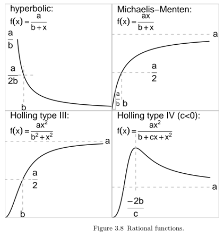
   As we do non-linear model-fitting, we're relying on knowing a fair number of non-linear animals at "the function zoo" -- and why we'd choose one versus another. The important features, as we choose a "functional form" for a model, are things like

   1. asymptotic behavior
   2. inflection
   3. slope at the origin
   4. extrema

5. Our last topic was SIR models (models of infectious disease), inspired by our current predicament with Covid-19. These are systems with three populations (or more). The basic SIR models looks like this:

   \[ \frac{dS}{dt} = -\alpha S I\\ \frac{dI}{dt} = \alpha S I - \beta I\\ \frac{dR}{dt} = \beta I \]

We also discovered the value in "flattening the curve" of the primary infection (as well as the danger of "squashing the curve" -- so that it simply comes back later on; we need a certain level of infection to attain a certain level of "herd immunity", to keep the outbreak from breaking out....).

So there are realistic lessons that we can learn from our models -- I hope that you appreciate those lessons. For example, you may remember in lab 2 how we squashed down too hard on infectivity with the social distancing from 30 to 110 days -- we dropped the infectivity from .45 to .10 during that time.

What happened was that we just put off the epidemic. It's exactly what this expert is explaining in her discussion of Covid-19 (which I got in my email feed this morning):

Herd immunity in California? A Stanford expert on why we're nowhere close: Dr Yvonne Maldonado explains why claims about early spread have been overblown and misleading

At Stanford University, located in Silicon Valley, researchers have been tracking early spread by pooling samples from patients with upper respiratory symptoms. In an initial study, the scientists found the presence of Covid-19 before mid-February was low; only two out of nearly 3,000 people with respiratory symptoms in early 2020 were later found to have had Covid-19.

• Dr Yvonne Maldonado, epidemiologist and infectious disease specialist at Stanford Medicine, explained why the claims about early spread have been overblown and misleading. This conversation has been edited and condensed for clarity.

• Some have suggested there was an early surge of coronavirus circulating in the community in California before March. What do we know? I don't believe that, and I don't have any evidence of that happening. That opinion seems to be based on pure conjecture. The data that I have seen does not suggest that there was a surge in February. We didn't have a coronavirus test until 4 March. So I don't know how you could make a surge diagnosis. There was a possibility that there may have been people infected before that time, because we didn't have a test. But with the testing that was available, we didn't really start seeing positives until the very end of February and then ramping up in March.

• What does this mean for immunity in California? We're not "immune" in California, because we're already starting to get antibody tests, and we don't have a high rate of antibody prevalence in just the few tests that have been run. In the coming weeks, we plan to use our own Stanford tests to look at antibody levels, and we're just not going to see very high levels. As devastating as this epidemic is, around the world we estimate that about 5% or less of people have actually been infected.

• So how do we move forward? With a disease like this, you probably need somewhere on the order of 60% or more people to have immunity in order to prevent an epidemic [ael: my emphasis]. Right now, if we're at less than 5%; you would need at least ten- to twelve-fold that level. The only way to get there is to vaccinate people or else have horrific transmissions[ael: my emphasis -- let the disease "burn itself out"], and we can't do the latter. So we're going to have to continue some social distancing efforts.

Predator/prey lab video summaries:

1. Lab PP1: Logistic growth
2. Lab PP2: Lotka-Volterra
3. Lab PP3: Tyson, et al.

Here are the SIR lab summaries:

1. Lab SIR1: Basic dynamics
2. Lab SIR2: Flatten the curve
3. Lab SIR3: Corona in Italy

The exam will include a "timed portion" (which I hope you can begin at class time -- let me know if that's a problem), and a "take home" portion (involving an and/either/or of regression and InsightMaker).

Some good links that I might recommend (a few of which we'll focus on):

1. A great intro to many of the most important question: "When a new virus emerges, no one is immune. A highly transmissible virus, like the coronavirus behind the current pandemic, can spread like wildfire, quickly burning through the dry kindling of a totally naive population. But once enough people are immune, the virus runs into walls of immunity, and the pandemic peters out instead of raging ahead. Scientists call that the herd immunity threshold."

2. How epidemics like covid-19 end (and how to end them faster): A coronavirus causing a disease called covid-19 has infected more than 70,000 people since it was first reported in late 2019. To predict how big the epidemic could get, researchers are working to determine how contagious the virus is.

3. The SIR Model for Spread of Disease - Introduction (from the MAA).

   In particular, we will implement The SIR Model for Spread of Disease - The Differential Equation Model in InsightMaker.

4. Mathematics of the Corona outbreak, with Professor Tim Britton

   (An excellent introduction to SIR models, from both the infectious disease and mathematical sides)

   Questions:

   1. Where is the "calculus moment" in this video?

   2. How does Britton suggest breaking $R_0$ down into "actionable" pieces?

5. An on-line model developed by Ashleigh Tuite and David Fisman, Dalla Lana School of Public Health, University of Toronto

6. This one incorporates space into the model. These models are called "agent-based models".

7. Could Coronavirus Cause as Many Deaths as Cancer in the U.S.? Putting Estimates in Context

   This on-line estimator (i.e., a model!) allows one to estimate deaths, as well as death by age-category.

8. A nice R-based introduction to infectious diseases and nonlinear differential equations.

9. Use of a log-scale (which they take pains to explain) to illustrate deaths by country, updated daily. There is even a separate page at the New York Times to explain log plots: "A Different Way to Chart the Spread of Coronavirus: Those skyrocketing curves tell an alarming story. But logarithmic graphs can help reveal when the pandemic begins to slow."